Understanding Gradient Clipping (and How It Can Fix Exploding Gradients Problem)

Gradient Clipping solves one of the biggest problems that we have while calculating gradients in Backpropagation for a Neural Network. 

You see, in a backward pass, we calculate gradients of all weights and biases in order to converge our cost function. These gradients, and the way they are calculated, are the secret behind the success of Artificial Neural Networks in every domain. 

But every good thing comes with some sort of caveat. 

Gradients tend to encapsulate information they collect from the data, which also includes long-range dependencies in large text or multidimensional data. So, while calculating complex data, things can go south really quickly, and you’ll blow your next million-dollar model in the process. 

Luckily, you can solve it before it occurs (with gradient clipping) – let’s first look at the problem in-depth.

By the end of this article you’ll know:

• What is Gradient Clipping and how does it occur?
• Types of Clipping techniques
• How to implement it in Tensorflow and Pytorch
• Additional research for you to read

Might interest you

Vanishing and Exploding Gradients in Neural Network Models: Debugging, Monitoring, and Fixing

Common problems with backpropagation

The Backpropagation algorithm is the heart of all modern-day Machine Learning applications, and it’s ingrained more deeply than you think. 

Backpropagation calculates the gradients of the cost function w.r.t – the weights and biases in the network.

It tells you about all the changes you need to make to your weights to minimize the cost function (it’s actually -1*∇ to see the steepest decrease, and +∇ would give you the steepest increase in the cost function). 

Pretty cool, because now you get to adjust all the weights and biases according to the training data you have. Neat math, all good.

Vanishing gradients

What about deeper networks, like Deep Recurrent Networks? 

The translation of the effect of a change in cost function(C) to the weight in an initial layer, or the norm of the gradient, becomes so small due to increased model complexity with more hidden units, that it becomes zero after a certain point. 

This is what we call Vanishing Gradients. 

This hampers the learning of the model. The weights can no longer contribute to the reduction in cost function(C), and go unchanged affecting the network in the Forward Pass, eventually stalling the model.

Exploding gradients

On the other hand, the Exploding gradients problem refers to a large increase in the norm of the gradient during training. 

Such events are caused by an explosion of long-term components, which can grow exponentially more than short-term ones. 

This results in an unstable network that at best cannot learn from the training data, making the gradient descent step impossible to execute. 

arXiv:1211.5063 [cs.LG]: The objective function for highly nonlinear deep neural networks or for recurrent neural networks often contains sharp nonlinearities in parameter space resulting from the multiplication of several parameters. These nonlinearities give rise to very high derivatives in some places. When the parameters get close to such a cliff region, a gradient descent update can catapult the parameters very far, possibly losing most of the optimization work that had been done.

Deep dive into exploding gradients problem

For calculating gradients in a Deep Recurrent Networks we use something called Backpropagation through time (BPTT), where the recurrent model is represented as a deep multi-layer one (with an unbounded number of layers), and backpropagation is applied on the unrolled model.

In other words, it’s backpropagation on an unrolled RNN.

Unrolling recurrent neural networks in time by creating a copy of the model for each time step: 

We denote by a<t> the hidden state of the network at time t, by x<t> the input and ŷ<t> the output of the network at time t, and by C<t> the error obtained from the output at time t.

Let’s work through some equations and see the root where it all starts.

We will diverge from classical BPTT equations at this point, and re-write the gradients in order to better highlight the exploding gradients problem. 

These equations were obtained by writing the gradients in a sum-of-products form.

We will also break down our flow into two parts:

• Forward Pass
• Backward Pass

Forward Pass

First, let’s check what intermediate activations of neurons at timestep <t> will look like:

Eq: 1.1

W_rec represents the recurrent matrix that will carry the translative effect of previous timesteps.
W_in is the matrix that gets matmul operation by the current timestep data and b represents bias. 

An intermediate output at timestep <t> will look something like:

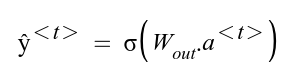
Eq: 1.2

Note that here “σ” represents any activation function of your choice. Popular picks include sigmoid, tanh, ReLU. 

Using the predicted and ground-truth value, we can calculate the Cost Function of the entire network by summing over individual Cost functions for every timestep <t>.

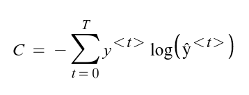
Eq: 1.3

Now, we have the general equations for the calculation of Cost Function. Let’s do a backward propagation, and see how gradients get calculated.

Backward Pass

In order to acquire the gradients from all timesteps, we again do a summation of all intermediate gradients at timestep <t>, and then the gradients are averaged over all training examples.

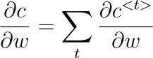
Eq: 1.4

So, we have to calculate the intermediate Cost Function(C) at any timestep <t> using the chain rule of derivatives. 

Let’s look at the dependency graph to identify the chain of derivatives:

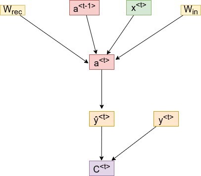
For a timestep <3>, our Cost Function will look something like:

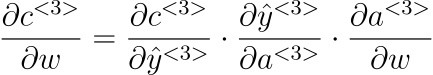
Eq: 1.5

Note: We’ve only mentioned derivative w.r.t to W which represents all the weights and bias matrices we’re trying to optimize.

As you can see above we get the activation a<3> which will depend on a<2>, and so on till the first layer’s activation is not calculated. 

Hence the dependency will go something like:

a<t> → a<t-1> → a<t-2> → …. → a<1>

So if we take the derivative with respect to W we can’t simply treat a<3> as constant. 

We need to apply the chain rule again. Finally, our equation will look something like this:

Eq: 1.6

We sum up the contributions of each time step to the gradient. 

In other words, because W is used in every step up to the output we care about, we need to backpropagate gradients from t=3 through the network all the way to t=0.

So, in order to calculate activation for a timestep <t>, we need all the activations from previous timesteps. 

Note that ∂a<T>/∂a<k> is a chain rule in itself! For example:

Eq: 1.7

Also note that because we are taking the derivative of a vector function with respect to a vector, the result is a matrix (called the Jacobian matrix) whose elements are all the pointwise derivatives. 

We can rewrite the above gradient in Eq:1.6:

Eq: 1.8

Eq: 1.9

This represents a Jacobian Matrix whose value is calculated using Frobenius or 2-norm. 

To understand this phenomenon we need to look at the form of each temporal component, and in particular at the matrix factors → ∂a<t>/ ∂a<k> (Eq:1.6,1.9) that take the form of a product of (t − k) Jacobian matrices. 

In the same way, a product of (t − k) real numbers can shrink to zero or explode to infinity, so does this product of matrices (along with some direction v). 

Hence, we get the condition of Exploding Gradients due to this temporal component.

How to identify and catch Exploding Gradients?

The identification of these gradient problems is hard to comprehend before the training process is even started. 

When your network is a deep recurrent one, you have to: 

• constantly monitor the logs,
• record sudden jumps in the cost function 

This will tell you whether these jumps are frequent and if the norm of the gradient is increasing exponentially. 

The best way to do this is by monitoring logs in a visualization dashboard.

We’ll utilize neptune.ai’s awesome visualization and dashboarding of the logs to monitor the loss and other metrics which will help in the identification of Exploding gradients. You can head over to the detailed documentation mentioned below to set up your dashboard.

READ MORE

How to Get Started With Neptune

How to fix exploding gradients: gradient clipping

There are a couple of techniques that focus on Exploding Gradient problems.

One common approach is L2 Regularization which applies “weight decay” in the cost function of the network.

The regularization parameter gets bigger, the weights get smaller, effectively making them less useful, as a result making the model more linear. 

However, we’ll focus on a technique that’s far superior in terms of gaining results and easiness in implementation – Gradient Clipping.

What is gradient clipping?

Gradient Clipping is a method where the error derivative is changed or clipped to a threshold during backward propagation through the network, and using the clipped gradients to update the weights. 

By rescaling the error derivative, the updates to the weights will also be rescaled, dramatically decreasing the likelihood of an overflow or underflow.

Effect of gradient clipping in a recurrent network with two parameters w and b. Gradient clipping can make gradient descent perform more reasonably in the vicinity of extremely steep cliffs. (Left)Gradient descent without gradient clipping overshoots the bottom of this small ravine, then receives a very large gradient from the cliff face. (Right) Gradient descent with gradient clipping has a more moderate reaction to the cliff. While it does ascend the cliff face, the step size is restricted so that it cannot be propelled away from the steep region near the solution. Figure adapted from Pascanu et al. (2013).

Gradient Clipping is implemented in two variants:

• Clipping-by-value
• Clipping-by-norm

Gradient clipping-by-value

The idea behind clipping-by-value is simple. We define a minimum clip value and a maximum clip value. 

If a gradient exceeds some threshold value, we clip that gradient to the threshold. If the gradient is less than the lower limit then we clip that too, to the lower limit of the threshold. 

The algorithm is as follows:

g ← ∂C/∂W

if ‖g‖ ≥ max_threshold or ‖g‖ ≤ min_threshold then

 g ← threshold (accordingly)

   end if

where max_threshold and min_threshold are the boundary values and between them lies a range of values that gradients can take. g, here is the gradient, and ‖g‖ is the norm of g.

Gradient clipping-by-norm

The idea behind clipping-by-norm is similar to by-value. The difference is that we clip the gradients by multiplying the unit vector of the gradients with the threshold. 

The algorithm is as follows:

g ← ∂C/∂W

if ‖g‖ ≥ threshold then

   g ← threshold * g/‖g‖

   end if

where the threshold is a hyperparameter, g is the gradient, and ‖g‖ is the norm of g. Since g/‖g‖ is a unit vector, after rescaling the new g will have norm equal to threshold. Note that if ‖g‖ < c, then we don’t need to do anything,

Gradient clipping ensures the gradient vector g has norm at most equal to threshold. 

This helps gradient descent to have reasonable behavior even if the loss landscape of the model is irregular, most likely a cliff.

Gradient clipping in deep learning frameworks

Now we know why Exploding Gradients occur and how Gradient Clipping can resolve it. 

We also saw two different methods by virtue of which you can apply Clipping to your deep neural network. 

Let’s see an implementation of both Gradient Clipping algorithms in major Machine Learning frameworks like Tensorflow and Pytorch. 

We’ll employ the MNIST dataset which is an open-source digit classification data meant for Image Classification.

For the first part, we’ll do some data loading and processing which is common for both Tensorflow and Keras.

Data loading

import tensorflow as tf
from tensorflow.keras import Model, layers
import numpy as np
import tensorflow_datasets as tfds

print(tf.__version__)

import neptune
run = neptune.init_run(project='common/tf-keras-integration',
                   api_token='ANONYMOUS')

We recommend you install the latest version of Tensorflow 2 which at the time of writing this was 2.3.0, but this code will be compatible with any future version. Make sure you’re installed with 2.3.0 or higher. In this excerpt, we’ve imported the TensorFlow dependencies as usual, with NumPy as our matrix computation library. 

from tensorflow.keras.datasets import mnist

(x_train, y_train), (x_test, y_test) = mnist.load_data()
# Convert to float32.
x_train, x_test = np.array(x_train, np.float32), np.array(x_test, np.float32)
# Flatten images to 1-D vector of 784 features (28*28).
x_train, x_test = x_train.reshape([-1, 28, 28]), x_test.reshape([-1, num_features])
# Normalize images value from [0, 255] to [0, 1].
x_train, x_test = x_train / 255., x_test / 255.

# Use tf.data API to shuffle and batch data.
train_data = tf.data.Dataset.from_tensor_slices((x_train, y_train))
train_data = train_data.repeat().shuffle(5000).batch(batch_size).prefetch(1)

Now, let’s see how to implement Gradient Clipping by-value and by-norm in Tensorflow.

TensorFlow

# Create LSTM Model.
class Net(Model):
    # Set layers.
    def __init__(self):
        super(Net, self).__init__()
        # RNN (LSTM) hidden layer.
        self.lstm_layer = layers.LSTM(units=num_units)
        self.out = layers.Dense(num_classes)

    # Set forward pass.
    def __call__(self, x, is_training=False):
        # LSTM layer.
        x = self.lstm_layer(x)
        # Output layer (num_classes).
        x = self.out(x)
        if not is_training:
            # tf cross entropy expect logits without softmax, so only
            # apply softmax when not training.
            x = tf.nn.softmax(x)
        return x

# Build LSTM model.
network = Net()

We’ve created a simple 2-layer network with the Input layer of LSTM (RNN based unit) and output/logit layer as Dense.

Now, let’s define other hyperparameters and metric functions to monitor and analyze.

# Hyperparameters
num_classes = 10 # total classes (0-9 digits).
num_features = 784 # data features (img shape: 28*28).

# Training Parameters
learning_rate = 0.001
training_steps = 1000
batch_size = 32
display_step = 100

# Network Parameters
# MNIST image shape is 28*28px, we will then handle 28 sequences of 28 timesteps for every sample.
num_input = 28 # number of sequences.
timesteps = 28 # timesteps.
num_units = 32 # number of neurons for the LSTM layer.
# Cross-Entropy Loss.
# Note that this will apply 'softmax' to the logits.
def cross_entropy_loss(x, y):
    # Convert labels to int 64 for tf cross-entropy function.
    y = tf.cast(y, tf.int64)
    # Apply softmax to logits and compute cross-entropy.
    loss = tf.nn.sparse_softmax_cross_entropy_with_logits(labels=y, logits=x)
    # Average loss across the batch.
    return tf.reduce_mean(loss)

# Accuracy metric.
def accuracy(y_pred, y_true):
    # Predicted class is the index of highest score in prediction vector (i.e. argmax).
    correct_prediction = tf.equal(tf.argmax(y_pred, 1), tf.cast(y_true, tf.int64))
    return tf.reduce_mean(tf.cast(correct_prediction, tf.float32), axis=-1)

# Adam optimizer.
optimizer = tf.optimizers.Adam(learning_rate)

Note that we are using Cross-Entropy loss function with softmax at the logit layer since this is a classification problem. Feel free to tweak the hyperparameters and play around with it to better understand the flow.

Now, let’s define the Optimization function where we’ll calculate the gradients, loss, and optimize our weights. Note that here we’ll apply the gradient clipping.

# Optimization process. 
def run_optimization(x, y):
    # Wrap computation inside a GradientTape for automatic differentiation.
    with tf.GradientTape() as tape:
        # Forward pass.
        pred = network(x, is_training=True)
        # Compute loss.
        loss = cross_entropy_loss(pred, y)

    # Variables to update, i.e. trainable variables.
    trainable_variables = network.trainable_variables

    # Compute gradients.
    gradients = tape.gradient(loss, trainable_variables)

    # Clip-by-value on all trainable gradients
    gradients = [(tf.clip_by_value(grad, clip_value_min=-1.0, clip_value_max=1.0))
                                  for grad in gradients]


    # Update weights following gradients.
    optimizer.apply_gradients(zip(gradients, trainable_variables))

At Line:14 we applied the Gradient Clip-by-value by iterating over all the gradients calculated at Line:11. Tensorflow has an explicit function definition in its API to apply Clipping.

To implement Gradient Clip-by-norm just change the Line 14 with:

# clip-by-norm
gradients = [(tf.clip_by_norm(grad, clip_norm=2.0)) for grad in gradients]

Let’s define a training loop and log metrics:

# Run training for the given number of steps.
for step, (batch_x, batch_y) in enumerate(train_data.take(training_steps), 1):
    # Run the optimization to update W and b values.
    run_optimization(batch_x, batch_y)

    if step % display_step == 0:
        pred = lstm_net(batch_x, is_training=True)
        loss = cross_entropy_loss(pred, batch_y)
        acc = accuracy(pred, batch_y)

        run['monitoring/logs/loss'].log(loss)
        run['monitoring/logs/acc'].log(acc)

        print("step: %i, loss: %f, accuracy: %f" % (step, loss, acc))

Keras

Keras works as a wrapper around the TensorFlow API to make things easier to understand and implement. The Keras API lets you focus on the definition stuff and takes care of the Gradient calculation, Backpropagation in the background. Gradient Clipping can be as simple as passing a hyperparameter in a function. Let’s see the specifics.

from tensorflow.keras.layers import Dense, LSTM
from tensorflow.keras.models import Sequential
from tensorflow.keras.optimizers import SGD
from tensorflow.keras.callbacks import Callback

import neptune
from neptune.integrations.tensorflow_keras import NeptuneCallback

import neptune
run = neptune.init_run(project='common/tf-keras-integration',
                   api_token='ANONYMOUS')
# define model
# using the hparams of tensorflow
model = Sequential()
model.add(LSTM(units=num_units))
model.add(Dense(num_classes))

We’ll now declare the gradient clipping factor, and finally fit the model with Keras’ awesome “.fit” method.

# compile model
optimizer = SGD(lr=0.01, momentum=0.9, clipvalue=1.0)
model.compile(loss='binary_crossentropy', optimizer=optimizer)
# fit model
neptune_cbk = NeptuneCallback(run=run, base_namespace='metrics')
history = model.fit(train_data, epochs=5, verbose=1,steps_per_epoch=training_steps,callbacks=[neptune_cbk])

Keras optimizers take care of additional gradient computation requests (like clipping in the background). Developers only need to pass values on these as hyperparameters.

In order to implement Clip-by-norm just alter the hyperparameter in Line:11 to:

# Gradient Clip-by-norm
optimizer = SGD(lr=0.01, momentum=0.9, clipnorm=1.0)

PyTorch

The implementation of Gradient Clipping, although algorithmically the same in both Tensorflow and Pytorch, is different in terms of flow and syntax. 

So, in this section of implementation with Pytorch, we’ll load data again, but now with Pytorch DataLoader class, and use the pythonic syntax to calculate gradients and clip them using the two methods we studied.

import os
import argparse
import torch
import torch.nn as nn
import torch.nn.functional as F
import torch.optim as optim
import torchvision
from torch.optim.lr_scheduler import StepLR

import neptune

import neptune
run = neptune.init_run(project='common/pytorch-integration',
                   api_token='ANONYMOUS')

Now, let’s declare some hyperparameters and DataLoader class in PyTorch.

# Hyperparameters
n_epochs = 2
batch_size_train = 64
batch_size_test = 1000
learning_rate = 0.01
momentum = 0.5
log_interval = 10

random_seed = 1
torch.backends.cudnn.enabled = False
torch.manual_seed(random_seed)

# Device configuration
device = torch.device('cuda' if torch.cuda.is_available() else 'cpu')

sequence_length = 28
input_size = 28
hidden_size = 128
num_layers = 2
num_classes = 10
batch_size = 100
num_epochs = 2
learning_rate = 0.01

os.makedirs('files',exist_ok=True)
train_loader = torch.utils.data.DataLoader(
  torchvision.datasets.MNIST('files/', train=True, download=True,
                             transform=torchvision.transforms.Compose([
                               torchvision.transforms.ToTensor(),
                               torchvision.transforms.Normalize(
                                 (0.1307,), (0.3081,))
                             ])),
  batch_size=batch_size_train, shuffle=True)

test_loader = torch.utils.data.DataLoader(
  torchvision.datasets.MNIST('files/', train=False, download=False,
                             transform=torchvision.transforms.Compose([
                               torchvision.transforms.ToTensor(),
                               torchvision.transforms.Normalize(
                                 (0.1307,), (0.3081,))
                             ])),
  batch_size=batch_size_test, shuffle=True)

Model time! we’ll declare the same model with LSTM as the input layer and Dense as the logit layer.

# Recurrent neural network (many-to-one)
class Net(nn.Module):
    def __init__(self, input_size, hidden_size, num_layers, num_classes):
        super(Net, self).__init__()
        self.hidden_size = hidden_size
        self.num_layers = num_layers
        self.lstm = nn.LSTM(input_size, hidden_size, num_layers, batch_first=True)
        self.fc = nn.Linear(hidden_size, num_classes)

    def forward(self, x):
        # Set initial hidden and cell states 
        h0 = torch.zeros(self.num_layers, x.size(0), self.hidden_size).to(device)
        c0 = torch.zeros(self.num_layers, x.size(0), self.hidden_size).to(device)

        # Forward propagate LSTM
        out, _ = self.lstm(x, (h0, c0))  # out: tensor of shape (batch_size, seq_length, hidden_size)

        # Decode the hidden state of the last time step
        out = self.fc(out[:, -1, :])
        return out


# Instantiate the model with hyperparameters
model = Net(input_size, hidden_size, num_layers, num_classes).to(device)

# Loss and optimizer
criterion = nn.CrossEntropyLoss()
optimizer = torch.optim.Adam(model.parameters(), lr=learning_rate)

Now, we’ll define the training loop in which gradient calculation along with optimizer steps will be defined. Here we’ll also define our clipping instruction.

# Train the model
total_step = len(train_loader)
for epoch in range(num_epochs):
    for i, (images, labels) in enumerate(train_loader):
        images = images.reshape(-1, sequence_length, input_size).to(device)
        labels = labels.to(device)

        # Forward pass
        outputs = model(images)
        loss = criterion(outputs, labels)

        # Backward and optimize
        optimizer.zero_grad()
        loss.backward()

        # Gradient Norm Clipping
        #nn.utils.clip_grad_norm_(model.parameters(), max_norm=2.0, norm_type=2)

        #Gradient Value Clipping
        nn.utils.clip_grad_value_(model.parameters(), clip_value=1.0)

        optimizer.step()

        run['monitoring/logs/loss'].log(loss)
        if (i+1) % 100 == 0:
            print ('Epoch [{}/{}], Step [{}/{}], Loss: {:.4f}'
                   .format(epoch+1, num_epochs, i+1, total_step, loss.item()))

Since PyTorch saves the gradients in the parameter name itself (a.grad), we can pass the model params directly to the clipping instruction. Line:17 describes how you can apply clip-by-value using torch’s clip_grad_value_ function. 

To apply Clip-by-norm you can change this line to:

# Gradient Norm Clipping
nn.utils.clip_grad_norm_(model.parameters(), max_norm=2.0, norm_type=2)

You can see the above metrics visualized here.

So, up to this point, you understand what clipping does and how to implement it. Now, in this section we’ll see it in action, sort of a before-after scenario to get you to understand the importance of it.

The framework of choice for this will be Pytorch since it has features to calculate norms on the fly and store it in variables.

Let’s start with the usual imports of dependencies.

import time
from tqdm import tqdm
import numpy as np
from sklearn.datasets import make_regression
import torch
import torch.nn as nn
import torch.nn.functional as F
import torch.optim as optim
from torchvision import datasets, transforms

import neptune
run = neptune.init_run(project='common/pytorch-integration',
                   api_token='ANONYMOUS')

For the sake of keeping the norms to handle small, we’ll only define two Linear/Dense layers for our neural network.

class Net(nn.Module):
    def __init__(self):
        super(Net, self).__init__()
        self.fc1 = nn.Linear(20, 25)
        self.fc2 = nn.Linear(25, 1)

        self.ordered_layers = [self.fc1,
                               self.fc2]
    def forward(self, x):
        x = F.relu(self.fc1(x))
        outputs = self.fc2(x)
        return outputs

We created “ordered_layers”variable in order to loop over them to extract norms.

def train_model(model,
                criterion,
                optimizer,
                num_epochs,
                with_clip=True):
    since = time.time()
    dataset_size = 1000

    for epoch in range(num_epochs):
        print('Epoch {}/{}'.format(epoch, num_epochs))
        print('-' * 10)
        time.sleep(0.1)
        model.train()  # Set model to training mode

        running_loss = 0.0
        batch_norm = []

        # Iterate over data.
        for idx,(inputs,label) in enumerate(tqdm(train_loader)):
            inputs = inputs.to(device)

            # zero the parameter gradients
            optimizer.zero_grad()

            # forward
            logits = model(inputs)
            loss = criterion(logits, label)

            # backward
            loss.backward()

            #Gradient Value Clipping
            if with_clip:
                nn.utils.clip_grad_value_(model.parameters(), clip_value=1.0)

            # calculate gradient norms
            for layer in model.ordered_layers:
                norm_grad = layer.weight.grad.norm()
                batch_norm.append(norm_grad.numpy())

            optimizer.step()

            # statistics
            running_loss += loss.item() * inputs.size(0)

        epoch_loss = running_loss / dataset_size

        if with_clip:
           run['monitoring/logs/grad_clipped'].log(np.mean(batch_norm))
        else:
            run['monitoring/logs/grad_nonclipped'].log(np.mean(batch_norm))

        print('Train Loss: {:.4f}'.format(epoch_loss))

        print()

    time_elapsed = time.time() - since
    print('Training complete in {:.0f}m {:.0f}s'.format(
        time_elapsed // 60, time_elapsed % 60))

This is a basic training function housing the main event loop that contains gradient calculations and optimizer steps. Here, we extract norms from the said “ordered_layers” variable. Now, we only have to initialize the model and call this function.

def init_weights(m):
    if type(m) == nn.Linear:
        torch.nn.init.xavier_uniform(m.weight)
        m.bias.data.fill_(0.01)

if __name__ == "__main__":
    device = torch.device("cpu")

    # prepare data
    X,y = make_regression(n_samples=1000, n_features=20, noise=0.1, random_state=1)

    X = torch.Tensor(X)
    y = torch.Tensor(y)

    dataset = torch.utils.data.TensorDataset(X,y)
    train_loader = torch.utils.data.DataLoader(dataset=dataset,batch_size=128, shuffle=True)

    model = Net().to(device)
    model.apply(init_weights)
    optimizer = optim.SGD(model.parameters(), lr=0.07, momentum=0.8)
    criterion = nn.MSELoss()

    norms = train_model(model=model,
                        criterion=criterion,
                        optimizer=optimizer,
                        num_epochs=50,
                        with_clip=True #make it False for without clipping
                        )

This will create a chart for the metrics you specified which will look something like this:

You can see the discrepancy between norms with and without clipping. During experiments without clipping, the norms exploded to NaN after a few epochs whereas experiments with clipping were fairly stable and converging. You can see the Neptune experiment here and the source code in the colab notebook here.

You’ve reached the end!

Congratulations! You’ve successfully understood the Gradient Clipping Methods, what problem it solves, and the Exploding Gradient Problem. 

Below are a few endnotes and future research things for you to follow through.

Logging is king!

Whenever you work on a big project with a large network, make sure that you are thorough with your logging procedures. 

Exploding Gradient can only be efficiently caught if you are logging and monitoring properly. 

You can use your current logging mechanisms in Tensorboard to visualize and monitor other metrics in Neptune’s dashboard. What you have to do is simply install neptune-client to accomplish that. Head over here to explore the documentation.

Research

• This paper explains how training speeds in Deep Networks can be enhanced using gradient clipping.
• This paper explains the use of Gradient clipping in differentially private neural networks.

That’s it for now, stay tuned for more! Adios!